SarcGraphTools - Visualization

All demos are availble on GitHub at https://github.com/Sarc-Graph/sarcgraph/tree/main/tutorials.

To run demos with jupyter notebook check Installation Guide.

SarcGraph includes the tools for visualization of recovered sarcomere characteristics.

In this notebook we provide a tutorial on how to use the SarcGraph package using demos and examples. The focus is on the SarcGraphTools.Visualization class in the sg_tools module.

Initialization

Run SarcGraphTools - Analysis Tutorial or t3-analysis.ipynb Before running this notebook. This will generate the following files in the directory specified by output_dir in the tutorial file:

• raw_frames.npy

• contours.npy

• sarcomeres_gpr.csv

• recovered_F.npy

• recovered_J.npy

• recovered_OOP.npy

• recovered_OOP_vector.npy

• recovered_metrics.json

• spatial-graph.pkl

• spatial-graph-pos.pkl

• time_series_params.csv

Create an instance of the sg_tools.SarcGraphTools class and set input_dir to the same directory that contains the above files:

from sarcgraph.sg_tools import SarcGraphTools

# Increase the quality to get better looking graphs
sg_tools = SarcGraphTools(input_dir='../tutorial-results', quality=50)

Visualization of Recovered Information

Here is a list of available functions in the SarcGraphTools.Visualization class:

• zdiscs_and_sarcs(): Visualizes detected z-discs and sarcomeres in one frame

• contraction(): Visualizes all detected sarcomeres in every frame saved as a gif file

• normalized_sarcs_length(): Plots normalized length of all sarcomeres versus frame number

• OOP(): Plots the recovered Orientational Order Parameter

• F(): Plots the recovered deformation gradient

• J(): Plots the recovered deformation gradient determinant

• F_eigenval_animation(): Visualizes the eigenvalues of U over all frames

• timeseries_params(): Visualizes timeseries parameters

• dendrogram(): Clusters timeseries and plots as a dendrogram of clusters

• spatial_graph(): Visualizes the spatial graph

• tracked_vs_untracked(): Visualizes some metrics to compare sarcomere detection with and without tracking

Note

Check the reference api for SarcGraphTools

Warning: Some of the functions may take a few minutes to run depending on the number of frames and sarcomeres.

Now, the functions listed above can be executed:

sg_tools.visualization.zdiscs_and_sarcs()

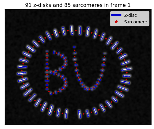
The figure will be saved as zdiscs-sarcs-frame-{frame_number}.png.

Note

For any png image an .eps file will also be saved if sg_tools.include_eps=True.

sg_tools.visualization.contraction()

GIF saved as '../tutorial-results/contract_anim.gif'!

To Visualize the GIF saved in the previous step, run the following:

import imageio
from IPython.display import display, Image

def read_gif_frames(file_path):
    with imageio.get_reader(file_path, format='GIF') as reader:
        frames = [frame for frame in reader]
    return frames

def display_gif_frames(frames):
    gif_bytes = imageio.mimwrite(imageio.RETURN_BYTES, frames, format='GIF')
    display(Image(data=gif_bytes))

# Read the frames from the existing GIF file
gif_path = '../tutorial-results/contract_anim.gif'
gif_frames = read_gif_frames(gif_path)

# Display the GIF using IPython.display
display_gif_frames(gif_frames)

<IPython.core.display.Image object>

sg_tools.visualization.normalized_sarcs_length()

The figure will be saved as normalized_sarcomeres_length.png.

sg_tools.visualization.OOP()

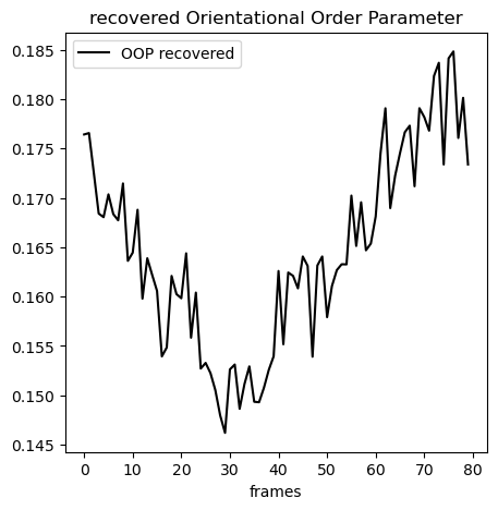
The figure will be saved as recovered_OOP.png.

sg_tools.visualization.F()

The figure will be saved as recovered_F.png.

sg_tools.visualization.J()

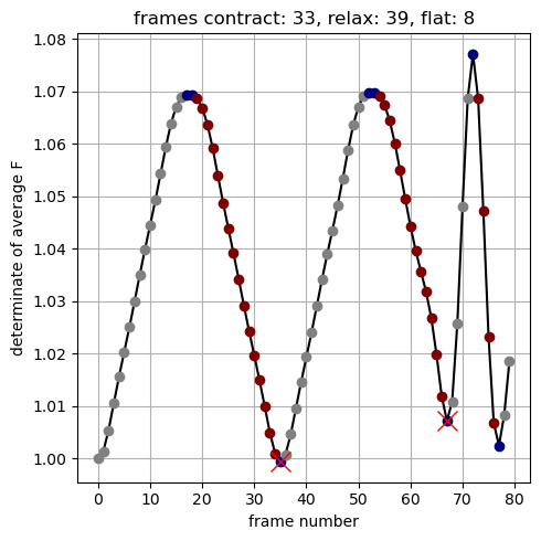
The figure will be saved as recovered_J.png.

sg_tools.visualization.F_eigenval_animation()

To visualize the GIF in jupyter notebook run the following:

import imageio
from IPython.display import display, Image

def read_gif_frames(file_path):
    with imageio.get_reader(file_path, format='GIF') as reader:
        frames = [frame for frame in reader]
    return frames

def display_gif_frames(frames):
    gif_bytes = imageio.mimwrite(imageio.RETURN_BYTES, frames, format='GIF')
    display(Image(data=gif_bytes))

# Read the frames from the existing GIF file
gif_path = '../tutorial-results/F_anim.gif'
gif_frames = read_gif_frames(gif_path)

# Display the GIF using IPython.display
display_gif_frames(gif_frames)

<IPython.core.display.Image object>

The animation will be saved as F_anim.gif.

sg_tools.visualization.timeseries_params()

The figure will be saved as histogram_time_constants.png.

sg_tools.visualization.dendrogram(dist_func="euclidean")
# you can switch to dist_func="dtw"

The figure will be saved as dendrogram_euclidean.pdf.

sg_tools.visualization.spatial_graph()

The figure will be saved as spatial-graph.png.

Note

tracked_vs_untracked() needs access to the original video/image file file_path.

sg_tools.visualization.tracked_vs_untracked('../samples/sample_1.avi', start_frame=10, stop_frame=50)

The figures will be saved as length-comparison.png, width-comparison.png, and angle-comparison.png.