SarcGraph Tutorial

All demos are availble on GitHub at https://github.com/Sarc-Graph/sarcgraph/tree/main/tutorials.

To run demos with jupyter notebook check Installation Guide.

SarcGraph incorporates functions to automatically detect and track z-discs and sarcomeres in movies of beating human induced pluripotent stem cell-derived cardiomyocytes (hiPSC-CMs). In addition, SarcGraph includes the tools which enable the recovery of basic sarcomere characteristics and the ability to run further high level analysis.

In this notebook we provide a tutorial on how to use the SarcGraph package using demos and examples. The focus if on the SarcGraph class in the sarcgraph.sg module.

SarcGraph on a Sample Video

In this section we show how to use SarcGraph to detect and track z-discs and sarcomeres in a sample movie of beating hiPSC-CM.

To showcase this we use samples/sample_0.avi.

Import Modules

The first step is to import SarcGraph class from sarcgraph module:

Note: If you are accessing this tutorial through Binder, please uncomment and run this cell.

# !pip install -e ../.

import numpy as np
import matplotlib.pyplot as plt
import pandas as pd

from sarcgraph import SarcGraph

SarcGraph Initialization

Next, we need to create an instance of the SarcGraph class.

After creating the instance, you will see a printed list of all configurable option variables.

You can change them using either of the two methods below:

```python sg.config.sigma = 2.0 sg._update_config(sigma=2.0)

sg = SarcGraph()

output_dir = output
input_type = video
save_output = True
sigma = 1.0
zdisc_min_length = 10
zdisc_max_length = 100
full_track_ratio = 0.75
tp_depth = 4
skip_merge = False
num_neighbors = 3
avg_sarc_length = 15.0
min_sarc_length = 0.0
max_sarc_length = 30.0
coeff_avg_length = 1.0
coeff_neighbor_length = 1.0
coeff_neighbor_angle = 1.0
score_threshold = 0.1
angle_threshold = 1.2

print("Original sigma:", sg.config.sigma)

sg.config.sigma = 2.0
print("Updated sigma (via direct assignment):", sg.config.sigma)

sg._update_config(sigma=3.0)
print("Updated sigma (via _update_config):", sg.config.sigma)

Original sigma: 1.0
Updated sigma (via direct assignment): 2.0
Updated sigma (via _update_config): 3.0

Run Detection

The simplest way to perform sarcomere detection on the video sample is to run SarcGraph().sarcomere_detection function:

sarcomeres, _ = sg.sarcomere_detection(input_file='../samples/sample_0.avi', input_type='video', sigma=1.0)

Frame 79: 81 trajectories present.

Note: Any keyword argument passed to a function like sarcomere_detection (e.g., sigma=2.0) is internally forwarded to sg._update_config(…) before the function runs. This lets you override config values without manually changing sg.config.

SarcGraph().sarcomere_detection automatically runs in three steps:

1. Z-disc segmentation: load the video, filter frames, and detect z-discs

2. Z-disc tracking: track detected z-discs

3. Sarcomere detection: detect sarcomeres using tracked z-discs information

And, this is how the output looks like:

Note

sarcomeres.sample(5) randomly picks 5 samples to display, and running the cell multiple times should output different results.

sarcomeres.sample(5)

	frame	sarc_id	x	y	length	width	angle	zdiscs
3529	9	44	122.827395	93.097301	19.091258	13.243788	0.633543	43,63
1494	54	18	202.852530	100.594535	21.386733	13.067663	0.585633	11,15
3543	23	44	119.437507	88.133541	20.331353	14.011109	0.642878	43,63
2616	56	32	274.940081	221.315493	12.413677	14.261831	1.663814	27,31
2693	53	33	276.983419	165.536505	12.977938	12.943811	1.812994	28,32

By dafault save_output=True in sg.config and the following information will be saved in sg.config.output_dir:

• raw video frames (grayscale)

• filtered video frames

• zdisc contours

• segmented zdiscs information

• tracked zdiscs information

• detected sarcomeres information

Simple Visualization

We briefly show how to use the saved information to visualize z-discs and sarcomeres in one frame of the video.

# load the information
output_dir = sg.config.output_dir
raw_frame = np.load(f"{output_dir}/raw_frames.npy")
tracked_zdiscs = pd.read_csv(f"{output_dir}/tracked_zdiscs.csv", index_col=[0])

frame_num = 0
sarcs_frame = sarcomeres[sarcomeres.frame == frame_num]
zdiscs_frame = tracked_zdiscs[tracked_zdiscs.frame == frame_num]

plt.figure(figsize=(7,7))
plt.axes().set_title(f'Sarcomeres and Z-Discs in Frame {frame_num}')
plt.axis('off')
plt.imshow(raw_frame[frame_num], cmap='gray')
plt.plot(zdiscs_frame.y, zdiscs_frame.x, 'r.', label='Z-Discs')
plt.plot(sarcs_frame.y, sarcs_frame.x, 'b.', ms=10, label='Sarcomeres')
plt.legend()

<matplotlib.legend.Legend at 0x722803f10910>

Alternative Way to Run SarcGraph

As mentioned in section Run Detection, sg.sarcomere_detection performs three tasks consecutively. Each task can also be run separately. Note that the results will not be saved since we have set save_output=False. We show how this can be done below:

Z-disc Segmentation

Run sg.zdisc_segmentation().

• Input could be either input_file or raw_frames.

Notes

• SarcGraph uses scikit library to load video/image files and can handle most formats. Yet, we recommend loading your sample video/image into a numpy array and pass the array as the input to SarcGraph functions, especially if the video/image is saved as a TIFF file.

zdiscs = sg.zdisc_segmentation(input_file='../samples/sample_0.avi', save_output=False)

# load `raw_frames`
# zdiscs = sg.zdisc_segmentation(raw_frames=raw_frame)

Z-disc Tracking

Run sg.zdisc_tracking().

• If the input is either input_file or raw_frames, this function runs sg.zdisc_segmentation first and then applies tracking.

• If the input is segmented_zdiscs, sg.zdisc_tracking only runs tracking.

tracked_zdiscs = sg.zdisc_tracking(segmented_zdiscs=zdiscs)

Frame 79: 81 trajectories present.

Let’s check the information stored in tracked_zdiscs:

tracked_zdiscs.sample(10)

	frame	x	y	p1_x	p1_y	p2_x	p2_y	particle	freq
1555	19	184.518660	266.525160	184.000000	260.667142	185.000000	272.718936	16	80
6429	79	184.506730	167.002881	182.000000	161.092676	187.000000	172.969227	39	80
2867	35	240.177834	150.183357	244.342161	146.000000	236.405462	155.000000	18	80
4018	49	111.995258	155.041922	108.000000	149.557462	115.000000	161.673055	42	80
4072	50	184.520292	277.996214	185.000000	270.838921	184.000000	285.085043	16	80
4251	52	270.681829	163.988891	273.000000	157.839894	269.000000	170.084687	32	80
3189	39	268.891087	263.511588	269.000000	256.284766	269.000000	270.835488	26	80
1480	18	184.714017	169.777278	182.000000	164.528144	187.000000	175.127891	39	80
2924	36	227.753694	148.106487	230.000000	142.209049	226.000000	153.472227	2	80
787	9	72.580198	100.578969	78.000000	96.474222	67.000000	104.803693	0	80

Sarcomere Detection Step

Run sg.sarcomere_detection().

• If the input is either input_file or raw_frames, this function runs sg.zdisc_segmentation then sg.zdisc_tracking before applying sarcomere detection.

• If the input is segmented_zdiscs, this function runs sg.zdisc_tracking first and then sarcomere detection.

• If the input is tracked_zdiscs, this function only runs sarcomere detection.

sarcs, _ = sg.sarcomere_detection(tracked_zdiscs=tracked_zdiscs)

SarcGraph on a Sample Image

To analyze a single frame, we can follow the same steps with a few modifications:

• When working on single-frame images instead of videos, tracking cannot be performed. Therefore, during SarcGraph Initialization, we should set input_type="image".

• If, instead of running SarcGraph().sarcomere_detection with input_file or raw_frames, you want to process the image step-by-step, you should still run SarcGraph().zdiscs_tracking or pass segmented_zdiscs into sarcomere_detection, even though tracking won’t be applied on still image.

Import SarcGraph class first:

from sarcgraph import SarcGraph

Create a new instance of SarcGraph class and set input_type='image'

sg_img = SarcGraph(output_dir='../tutorial-results-image', input_type='image')

output_dir = ../tutorial-results-image
input_type = image
save_output = True
sigma = 1.0
zdisc_min_length = 10
zdisc_max_length = 100
full_track_ratio = 0.75
tp_depth = 4
skip_merge = False
num_neighbors = 3
avg_sarc_length = 15.0
min_sarc_length = 0.0
max_sarc_length = 30.0
coeff_avg_length = 1.0
coeff_neighbor_length = 1.0
coeff_neighbor_angle = 1.0
score_threshold = 0.1
angle_threshold = 1.2

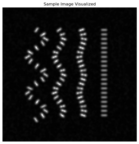
Let’s load a sample image to a numpy array and pass it to sg_img.sarcomere_detection() rather than specifying input_file:

Note

We used matplotlib.image to load the image here.

import matplotlib

img = matplotlib.image.imread('../samples/sample_5.png')

plt.figure(figsize=(7,7))
plt.axes().set_title('Sample Image Visualized')
plt.axis('off')
plt.imshow(img, cmap='gray')

<matplotlib.image.AxesImage at 0x7228020eb190>

Now we can run sg_img.sarcomere_detection():

# Image must be a stack of 2D images even if it is a single image.
img = img[None, :, :]
sarcs_img, _ = sg_img.sarcomere_detection(raw_frames=img)

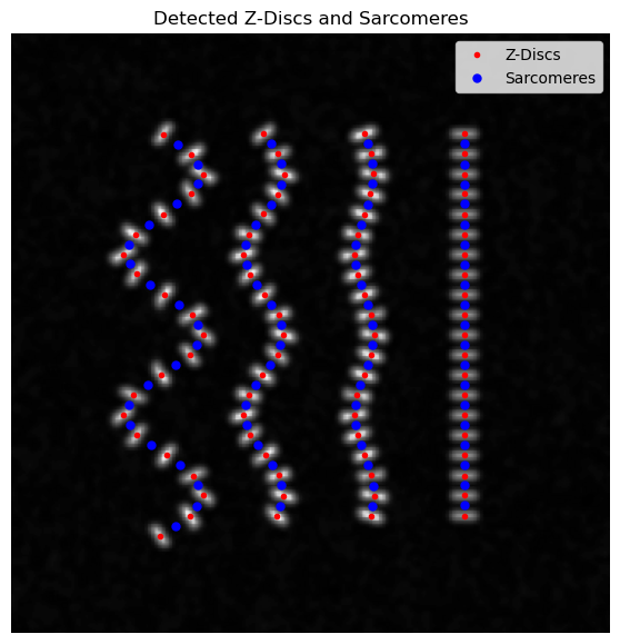
Similar to the video sample, we will visualize detected sarcomeres in this image:

output_dir = sg_img.config.output_dir

segmented_zdiscs = pd.read_csv(f"{output_dir}/segmented_zdiscs.csv", index_col=[0])

plt.figure(figsize=(7,7))
plt.axes().set_title('Detected Z-Discs and Sarcomeres')
plt.axis('off')
plt.imshow(img[0], cmap='gray')
plt.plot(segmented_zdiscs.y, segmented_zdiscs.x, 'r.', label='Z-Discs')
plt.plot(sarcs_img.y, sarcs_img.x, 'b.', ms=10, label='Sarcomeres')
plt.legend()

<matplotlib.legend.Legend at 0x72280a66ed40>