SarcGraph Tutorial

All demos are availble on GitHub at https://github.com/Sarc-Graph/sarcgraph/tree/main/tutorials.

To run demos with jupyter notebook check Installation Guide.

SarcGraph incorporates functions to automatically detect and track z-discs and sarcomeres in movies of beating human induced pluripotent stem cell-derived cardiomyocytes (hiPSC-CMs). In addition, SarcGraph includes the tools which enable the recovery of basic sarcomere characteristics and the ability to run further high level analysis.

In this notebook we provide a tutorial on how to use the SarcGraph package using demos and examples. The focus if on the SarcGraph class in the sarcgraph.sg module.

SarcGraph on a Sample Video

In this section we show how to use SarcGraph to detect and track z-discs and sarcomeres in a sample movie of beating hiPSC-CM.

To showcase this we use samples/sample_0.avi.

Import Modules

The first step is to import SarcGraph class from sarcgraph.sg module:

Note: If you are accessing this tutorial through Binder, please uncomment and run this cell.

# !pip install -e ../.

import numpy as np
import matplotlib.pyplot as plt
import pandas as pd

from sarcgraph.sg import SarcGraph

SarcGraph Initialization

Next we need to create an instance of SarcGraph class:

SarcGraph class takes two optional inputs: - output_dir: the directory to save the results - default: 'test-run' - file_type: whether the sample is a video or an image - default: 'video'

sg = SarcGraph(output_dir='../tutorial-results', file_type='video')

Run Detection

The simplest way to perform sarcomere detection on the video sample is to run SarcGraph().sarcomere_detection function:

sarcomeres, _ = sg.sarcomere_detection(file_path='../samples/sample_0.avi')

Frame 79: 81 trajectories present.

SarcGraph().sarcomere_detection automatically runs in three steps:

1. Z-disc segmentation: load the video, filter frames, and detect z-discs

2. Z-disc tracking: track detected z-discs

3. Sarcomere detection: detect sarcomeres using tracked z-discs information

And, this is how the output looks like:

Note

sarcomeres.sample(5) randomly picks 5 samples to display, and running the cell multiple times should output different results.

sarcomeres.sample(5)

	frame	sarc_id	x	y	length	width	angle	zdiscs
220	60	2	278.646713	267.714240	11.397091	14.080775	0.000067	-1,26
4877	77	60	116.730978	214.462941	12.949554	14.099212	2.805399	59,79
2910	30	36	264.642071	218.846934	13.029619	13.280433	0.318365	31,35
3830	70	47	113.105042	267.712294	11.226317	13.896309	0.002197	44,60
219	59	2	280.124606	270.096786	10.119645	14.683792	0.003224	-1,26

By dafault save_output=True in sg.sarcomere_detection() and the following information will be saved in sg.output_dir:

• raw video frames (grayscale)

• filtered video frames

• zdisc contours

• segmented zdiscs information

• tracked zdiscs information

• detected sarcomeres information

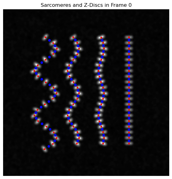
Simple Visualization

We briefly show how to use the saved information to visualize z-discs and sarcomeres in one frame of the video.

# load the information
raw_frame = np.load(f"{sg.output_dir}/raw-frames.npy")[0, :, :, 0]
tracked_zdiscs = pd.read_csv(f"{sg.output_dir}/tracked-zdiscs.csv", index_col=[0])

sarcs_frame = sarcomeres[sarcomeres.frame == 0]
zdiscs_frame = tracked_zdiscs[tracked_zdiscs.frame == 0]

plt.figure(figsize=(7,7))
plt.axes().set_title('Sarcomeres and Z-Discs in Frame 0')
plt.axis('off')
plt.imshow(raw_frame, cmap='gray')
plt.plot(zdiscs_frame.y, zdiscs_frame.x, 'r.')
plt.plot(sarcs_frame.y, sarcs_frame.x, 'b.', ms=10)

[<matplotlib.lines.Line2D at 0x285ad65b160>]

Alternative Way to Run SarcGraph

As mentioned in section Run Detection, sg.sarcomere_detection performs three tasks consecutively. Each task can also be run separately. Note that the results will not be saved since we have set save_output=False. We show how this can be done below:

Z-disc Segmentation

Run sg.zdisc_segmentation().

• Input could be either file_path or raw_frames.

Notes

• raw_frames must be a 4d numpy array with shape=(frames, dim 1, dim 2, channels), for example, for a grayscale video with 20 frames and resolution of 400x400 the shape of raw_frames is (20, 400, 400, 1)

• SarcGraph uses scikit library to load video/image files and can handle most formats. Yet, we recommend loading your sample video/image into a numpy array and pass the array as the input to SarcGraph functions, especially if the video/image is saved as a TIFF file.

zdiscs = sg.zdisc_segmentation(file_path='../samples/sample_0.avi', save_output=False)

Z-disc Tracking

Run sg.zdisc_tracking().

• If the input is either file_path or raw_frames, this function runs sg.zdisc_segmentation first and then applies tracking.

• If the input is segmented_zdiscs, sg.zdisc_tracking only runs tracking.

tracked_zdiscs = sg.zdisc_tracking(segmented_zdiscs=zdiscs, save_output=False)

Frame 79: 81 trajectories present.

Let’s check the information stored in tracked_zdiscs:

tracked_zdiscs.sample(10)

	frame	x	y	p1_x	p1_y	p2_x	p2_y	particle	freq
3270	40	279.114063	166.565872	275.000000	160.430515	283.000000	172.113936	24	80
1661	20	184.597237	169.178027	182.000000	163.418879	187.000000	174.990273	39	80
770	9	173.353513	217.482265	174.000000	212.414066	172.000000	222.388170	62	80
968	11	141.369782	146.787244	144.000000	141.701820	139.000000	152.430764	76	80
5919	72	138.771012	76.135783	142.000000	70.795997	135.000000	81.007262	77	80
4286	52	159.956104	278.157040	160.000000	270.661829	160.000000	285.328813	66	80
488	6	232.340605	210.864295	234.000000	204.086232	232.000000	217.365572	1	80
1356	16	121.575798	159.141550	118.000000	152.555463	125.000000	165.887396	42	80
1321	16	279.379684	166.246376	274.901385	160.000000	283.047762	172.000000	24	80
3214	39	100.737593	127.985250	98.000000	122.160055	103.000000	132.979194	51	80

Sarcomere Detection Step

Run sg.sarcomere_detection().

• If the input is either file_path or raw_frames, this function runs sg.zdisc_segmentation then sg.zdisc_tracking before applying sarcomere detection.

• If the input is segmented_zdiscs, this function runs sg.zdisc_tracking first and then sarcomere detection.

• If the input is tracked_zdiscs, this function only runs sarcomere detection.

sarcs, _ = sg.sarcomere_detection(tracked_zdiscs=tracked_zdiscs)

SarcGraph on a Sample Image

To analyze a single frame we can follow the steps with a few changes:

• When we are working on single-frame images and not videos, the tracking part cannot be done! Therefore, during SarcGraph Initialization we should set file_type="image".

• If rather than running SarcGraph().sarcomere_detection, we need to process the image step by step, we should still run SarcGraph().zdiscs_tracking although it does not do much.

Import SarcGraph class first:

from sarcgraph.sg import SarcGraph

Create a new instance of SarcGraph class and set file_type='image'

sg_img = SarcGraph(output_dir='../tutorial-results-image', file_type='image')

Let’s load a sample image to a numpy array and pass it to sg_img.sarcomere_detection() rather than specifying file_path:

Note

We used matplotlib.image to load the image here.

import matplotlib

img = matplotlib.image.imread('../samples/sample_5.png')

plt.figure(figsize=(7,7))
plt.axes().set_title('Sample Image Visualized')
plt.axis('off')
plt.imshow(img, cmap='gray')

<matplotlib.image.AxesImage at 0x285ad6bd420>

Our sample image has the shape (368, 368) which needs to be reshaped to (1, 368, 368, 1) - [frames, dimension 1, dimension 2, color channels].

img = img[None, :, :, None]

Now we can run sg_img.sarcomere_detection():

sarcs_img, _ = sg_img.sarcomere_detection(raw_frames=img)

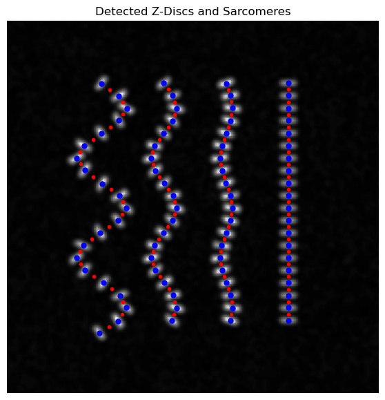
Similar to the video sample, we will visualize detected sarcomeres in this image:

segmented_zdiscs = pd.read_csv(f"{sg_img.output_dir}/segmented-zdiscs.csv", index_col=[0])

plt.figure(figsize=(7,7))
plt.axes().set_title('Detected Z-Discs and Sarcomeres')
plt.axis('off')
plt.imshow(img[0, :, :, 0], cmap='gray')
plt.plot(sarcs_img.y, sarcs_img.x, 'r.')
plt.plot(segmented_zdiscs.y, segmented_zdiscs.x, 'b.', ms=10)

[<matplotlib.lines.Line2D at 0x285ad34d090>]